Dfyjkt

chi-squared
	; Probability density function;
	; Cumulative distribution function;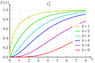
Notation	; χ2(k)displaystyle chi ^2(k); or χk2displaystyle chi _k^2!;
Parameters	; k∈N>0 displaystyle kin mathbb N _>0~~ (known as "degrees of freedom")
Support	; x∈(0,+∞)displaystyle xin (0,+infty ); if k=1displaystyle k=1, otherwise x∈[0,+∞)displaystyle xin [0,+infty );;
PDF	12k/2Γ(k/2)xk/2−1e−x/2displaystyle frac 12^k/2Gamma (k/2);x^k/2-1e^-x/2;
CDF	1Γ(k/2)γ(k2,x2)displaystyle frac 1Gamma (k/2);gamma left(frac k2,,frac x2right);
Mean	kdisplaystyle k
Median	≈k(1−29k)3displaystyle approx kbigg (1-frac 29kbigg )^3;
Mode	max(k−2,0)displaystyle max(k-2,0);
Variance	2kdisplaystyle 2k;
Skewness	8/kdisplaystyle scriptstyle sqrt 8/k,
Ex. kurtosis	12kdisplaystyle frac 12k
Entropy	k2+log⁡(2Γ(k/2))+(1−k/2)ψ(k/2)(nats)displaystyle beginalignedtfrac k2&+log(2Gamma (k/2))\&!+(1-k/2)psi (k/2),scriptstyle text(nats)endaligned
MGF	(1−2t)−k/2 for t<12displaystyle (1-2t)^-k/2text for t<frac 12;
CF	; (1−2it)−k/2displaystyle (1-2it)^-k/2
PGF	(1−2ln⁡t)−k/2 for 0<t<edisplaystyle (1-2ln t)^-k/2text for 0<t<sqrt e;

In probability theory and statistics, the chi-squared distribution (also chi-square or χ²-distribution) with $k$ degrees of freedom is the distribution of a sum of the squares of $k$ independent standard normal random variables. The chi-squared distribution is a special case of the gamma distribution and is one of the most widely used probability distributions in inferential statistics, notably in hypothesis testing or in construction of confidence intervals.^[2]^[3]^[4]^[5] When it is being distinguished from the more general noncentral chi-squared distribution, this distribution is sometimes called the central chi-squared distribution.

The chi-squared distribution is used in the common chi-squared tests for goodness of fit of an observed distribution to a theoretical one, the independence of two criteria of classification of qualitative data, and in confidence interval estimation for a population standard deviation of a normal distribution from a sample standard deviation. Many other statistical tests also use this distribution, such as Friedman's analysis of variance by ranks.

Definition

If Z₁, ..., Z_k are independent, standard normal random variables, then the sum of their squares,

Q =sum _i=1^kZ_i^2,

is distributed according to the chi-squared distribution with k degrees of freedom. This is usually denoted as

Q sim chi ^2(k) textor Q sim chi _k^2.

The chi-squared distribution has one parameter: k, a positive integer that specifies the number of degrees of freedom (the number of Z_i’s).

Introduction

The chi-squared distribution is used primarily in hypothesis testing, and to a lesser extent for confidence intervals for population variance when the underlying distribution is normal. Unlike more widely known distributions such as the normal distribution and the exponential distribution, the chi-squared distribution is not as often applied in the direct modeling of natural phenomena. It arises in the following hypothesis tests, among others.

Chi-squared test of independence in contingency tables

Chi-squared test of goodness of fit of observed data to hypothetical distributions

Likelihood-ratio test for nested models

Log-rank test in survival analysis

Cochran–Mantel–Haenszel test for stratified contingency tables

It is also a component of the definition of the t-distribution and the F-distribution used in t-tests, analysis of variance, and regression analysis.

The primary reason that the chi-squared distribution is used extensively in hypothesis testing is its relationship to the normal distribution. Many hypothesis tests use a test statistic, such as the t-statistic in a t-test. For these hypothesis tests, as the sample size, n, increases, the sampling distribution of the test statistic approaches the normal distribution (central limit theorem). Because the test statistic (such as t) is asymptotically normally distributed, provided the sample size is sufficiently large, the distribution used for hypothesis testing may be approximated by a normal distribution. Testing hypotheses using a normal distribution is well understood and relatively easy. The simplest chi-squared distribution is the square of a standard normal distribution. So wherever a normal distribution could be used for a hypothesis test, a chi-squared distribution could be used.

Specifically, suppose that Z is a standard normal random variable, with mean = 0 and variance = 1. Z ~ N(0,1). A sample drawn at random from Z is a sample from the distribution shown in the graph of the standard normal distribution.
Define a new random variable Q. To generate a random sample from Q, take a sample from Z and square the value. The distribution of the squared values is given by the random variable Q = Z². The distribution of the random variable Q is an example of a chi-squared distribution: $Q sim chi _1^2.$ The subscript 1 indicates that this particular chi-squared distribution is constructed from only 1 standard normal distribution. A chi-squared distribution constructed by squaring a single standard normal distribution is said to have 1 degree of freedom. Thus, as the sample size for a hypothesis test increases, the distribution of the test statistic approaches a normal distribution, and the distribution of the square of the test statistic approaches a chi-squared distribution. Just as extreme values of the normal distribution have low probability (and give small p-values), extreme values of the chi-squared distribution have low probability.

An additional reason that the chi-squared distribution is widely used is that it is a member of the class of likelihood ratio tests (LRT).^[6] LRT's have several desirable properties; in particular, LRT's commonly provide the highest power to reject the null hypothesis (Neyman–Pearson lemma). However, the normal and chi-squared approximations are only valid asymptotically. For this reason, it is preferable to use the t distribution rather than the normal approximation or the chi-squared approximation for small sample size. Similarly, in analyses of contingency tables, the chi-squared approximation will be poor for small sample size, and it is preferable to use Fisher's exact test. Ramsey shows that the exact binomial test is always more powerful than the normal approximation.^[7]

Lancaster shows the connections among the binomial, normal, and chi-squared distributions, as follows.^[8] De Moivre and Laplace established that a binomial distribution could be approximated by a normal distribution. Specifically they showed the asymptotic normality of the random variable

displaystyle chi =m-Np over sqrt Npq

where m is the observed number of successes in N trials, where the probability of success is p, and q = 1 − p.

Squaring both sides of the equation gives

displaystyle chi ^2=(m-Np)^2 over Npq

Using N = Np + N(1 − p), N = m + (N − m), and q = 1 − p, this equation simplifies to

displaystyle chi ^2=(m-Np)^2 over Np+(N-m-Nq)^2 over Nq

The expression on the right is of the form that Pearson would generalize to the form:

displaystyle chi ^2=sum _i=1^nfrac (O_i-E_i)^2E_i

where

chi ^2

= Pearson's cumulative test statistic, which asymptotically approaches a

chi ^2

distribution.

O_i

= the number of observations of type i.

E_i=Np_i

= the expected (theoretical) frequency of type i, asserted by the null hypothesis that the fraction of type i in the population is

p_i

n

= the number of cells in the table.

In the case of a binomial outcome (flipping a coin), the binomial distribution may be approximated by a normal distribution (for sufficiently large n). Because the square of a standard normal distribution is the chi-squared distribution with one degree of freedom, the probability of a result such as 1 heads in 10 trials can be approximated either by the normal or the chi-squared distribution. However, many problems involve more than the two possible outcomes of a binomial, and instead require 3 or more categories, which leads to the multinomial distribution. Just as de Moivre and Laplace sought for and found the normal approximation to the binomial, Pearson sought for and found a multivariate normal approximation to the multinomial distribution. Pearson showed that the chi-squared distribution, the sum of multiple normal distributions, was such an approximation to the multinomial distribution ^[8]

Characteristics

Further properties of the chi-squared distribution can be found in the box at the upper right corner of this article.

Probability density function

The probability density function (pdf) of the chi-square distribution is

displaystyle f(x;,k)=begincasesdfrac x^frac k2-1e^-frac x22^frac k2Gamma left(frac k2right),&x>0;\0,&textotherwise.endcases

where $textstyle Gamma (k/2)$ denotes the gamma function, which has closed-form values for integer k.

For derivations of the pdf in the cases of one, two and k degrees of freedom, see Proofs related to chi-squared distribution.

Cumulative distribution function

Chernoff bound for the CDF and tail (1-CDF) of a chi-squared random variable with ten degrees of freedom (k = 10)

Its cumulative distribution function is:

F(x;,k)=frac gamma (frac k2,,frac x2)Gamma (frac k2)=Pleft(frac k2,,frac x2right),

where $displaystyle gamma (s,t)$ is the lower incomplete gamma function and $textstyle P(s,t)$ is the regularized gamma function.

In a special case of k = 2 this function has a simple form:^{[citation needed]}

displaystyle F(x;,2)=1-e^-x/2

and the integer recurrence of the gamma function makes it easy to compute for other small even k.

Tables of the chi-squared cumulative distribution function are widely available and the function is included in many spreadsheets and all statistical packages.

Letting $zequiv x/k$ , Chernoff bounds on the lower and upper tails of the CDF may be obtained.^[9] For the cases when $0<z<1$ (which include all of the cases when this CDF is less than half):

F(zk;,k)leq (ze^1-z)^k/2.

The tail bound for the cases when $z>1$ , similarly, is

1-F(zk;,k)leq (ze^1-z)^k/2.

For another approximation for the CDF modeled after the cube of a Gaussian, see under Noncentral chi-squared distribution.

Additivity

It follows from the definition of the chi-squared distribution that the sum of independent chi-squared variables is also chi-squared distributed. Specifically, if X_i_i=1ⁿ are independent chi-squared variables with k_i_i=1ⁿ degrees of freedom, respectively, then Y = X₁ + ⋯ + X_n is chi-squared distributed with k₁ + ⋯ + k_n degrees of freedom.

Sample mean

The sample mean of $n$ i.i.d. chi-squared variables of degree $k$ is distributed according to a gamma distribution with shape $alpha$ and scale $theta$ parameters:

displaystyle bar X=frac 1nsum _i=1^nX_isim operatorname Gamma left(alpha =n,k/2,theta =2/nright)qquad textwhere X_isim chi ^2(k)

Asymptotically, given that for a scale parameter $alpha$ going to infinity, a Gamma distribution converges towards a normal distribution with expectation $mu =alpha cdot theta$ and variance $sigma ^2=alpha ,theta ^2$ , the sample mean converges towards:

bar Xxrightarrow nto infty N(mu =k,sigma ^2=2,k/n)

Note that we would have obtained the same result invoking instead the central limit theorem, noting that for each chi-squared variable of degree $k$ the expectation is $k$ , and its variance $2,k$ (and hence the variance of the sample mean $bar X$ being $sigma ^2=2,k/n$ ).

Entropy

The differential entropy is given by

displaystyle h=int _0^infty f(x;,k)ln f(x;,k),dx=frac k2+ln left[2,Gamma left(frac k2right)right]+left(1-frac k2right),psi !left[frac k2right],

where ψ(x) is the Digamma function.

The chi-squared distribution is the maximum entropy probability distribution for a random variate X for which $displaystyle operatorname E (X)=k$ and $displaystyle operatorname E (ln(X))=psi (k/2)+ln(2)$ are fixed. Since the chi-squared is in the family of gamma distributions, this can be derived by substituting appropriate values in the Expectation of the log moment of gamma. For derivation from more basic principles, see the derivation in moment-generating function of the sufficient statistic.

Noncentral moments

The moments about zero of a chi-squared distribution with k degrees of freedom are given by^[10]^[11]

displaystyle operatorname E (X^m)=k(k+2)(k+4)cdots (k+2m-2)=2^mfrac Gamma left(m+frac k2right)Gamma left(frac k2right).

Cumulants

The cumulants are readily obtained by a (formal) power series expansion of the logarithm of the characteristic function:

kappa _n=2^n-1(n-1)!,k

Asymptotic properties

By the central limit theorem, because the chi-squared distribution is the sum of k independent random variables with finite mean and variance, it converges to a normal distribution for large k. For many practical purposes, for k > 50 the distribution is sufficiently close to a normal distribution for the difference to be ignored.^[12] Specifically, if X ~ χ²(k), then as k tends to infinity, the distribution of $(X-k)/sqrt 2k$ tends to a standard normal distribution. However, convergence is slow as the skewness is $sqrt 8/k$ and the excess kurtosis is 12/k.

The sampling distribution of ln(χ²) converges to normality much faster than the sampling distribution of χ²,^[13] as the logarithm removes much of the asymmetry.^[14] Other functions of the chi-squared distribution converge more rapidly to a normal distribution. Some examples are:

If X ~ χ²(k) then $scriptstyle sqrt 2X$ is approximately normally distributed with mean $scriptstyle sqrt 2k-1$ and unit variance (1922, by R. A. Fisher, see (18.23), p. 426 of.^[4]

If X ~ χ²(k) then $scriptstyle sqrt[3]X/k$ is approximately normally distributed with mean $scriptstyle 1-2/(9k)$ and variance $scriptstyle 2/(9k).$ ^[15] This is known as the Wilson–Hilferty transformation, see (18.24), p. 426 of.^[4]

Relation to other distributions

Approximate formula for median compared with numerical quantile (top). Difference between numerical quantile and approximate formula (bottom).

As $kto infty$ , $(chi _k^2-k)/sqrt 2k~xrightarrow d N(0,1),$ (normal distribution)

$chi _k^2sim chi '_k^2(0)$ (noncentral chi-squared distribution with non-centrality parameter $lambda =0$ )

If $displaystyle Ysim mathrm F (nu _1,nu _2)$ then $displaystyle X=lim _nu _2to infty nu _1Y$ has the chi-squared distribution $chi _nu _1^2$

As a special case, if $displaystyle Ysim mathrm F (1,nu _2),$ then $displaystyle X=lim _nu _2to infty Y,$ has the chi-squared distribution $chi _1^2$

$boldsymbol N_i=1,ldots ,k(0,1)$ (The squared norm of k standard normally distributed variables is a chi-squared distribution with k degrees of freedom)

If $displaystyle Xsim chi ^2(nu ),$ and $c>0,$ , then $displaystyle cXsim Gamma (k=nu /2,theta =2c),$ . (gamma distribution)

If $Xsim chi _k^2$ then $sqrt Xsim chi _k$ (chi distribution)

If $displaystyle Xsim chi ^2(2)$ , then $displaystyle Xsim operatorname Exp (1/2)$ is an exponential distribution. (See gamma distribution for more.)

If $displaystyle Xsim chi ^2(2k)$ , then $displaystyle Xsim operatorname Erlang (k,1/2)$ is an Erlang distribution.

If $displaystyle Xsim operatorname Erlang (k,lambda )$ , then $displaystyle 2lambda Xsim chi _2k^2$

If $displaystyle Xsim operatorname Rayleigh (1),$ (Rayleigh distribution) then $X^2sim chi ^2(2),$

If $displaystyle Xsim operatorname Maxwell (1),$ (Maxwell distribution) then $X^2sim chi ^2(3),$

If $Xsim chi ^2(nu )$ then $displaystyle tfrac 1Xsim operatorname Inv- chi ^2(nu ),$ (Inverse-chi-squared distribution)

The chi-squared distribution is a special case of type 3 Pearson distribution

If $Xsim chi ^2(nu _1),$ and $Ysim chi ^2(nu _2),$ are independent then $displaystyle tfrac XX+Ysim operatorname Beta (tfrac nu _12,tfrac nu _22),$ (beta distribution)

If $displaystyle Xsim operatorname U (0,1),$ (uniform distribution) then $displaystyle -2log(X)sim chi ^2(2),$

$chi ^2(6),$ is a transformation of Laplace distribution

If $displaystyle X_isim operatorname Laplace (mu ,beta ),$ then $displaystyle sum _i=1^nfrac 2beta sim chi ^2(2n),$

If $X_i$ follows the generalized normal distribution (version 1) with parameters $displaystyle mu ,alpha ,beta$ then $displaystyle sum _i=1^nfrac X_i-mu alpha sim chi ^2left(frac 2nbeta right),$ ^[16]

chi-squared distribution is a transformation of Pareto distribution

Student's t-distribution is a transformation of chi-squared distribution

Student's t-distribution can be obtained from chi-squared distribution and normal distribution

Noncentral beta distribution can be obtained as a transformation of chi-squared distribution and Noncentral chi-squared distribution

Noncentral t-distribution can be obtained from normal distribution and chi-squared distribution

A chi-squared variable with k degrees of freedom is defined as the sum of the squares of k independent standard normal random variables.

If Y is a k-dimensional Gaussian random vector with mean vector μ and rank k covariance matrix C, then X = (Y−μ)^TC⁻¹(Y − μ) is chi-squared distributed with k degrees of freedom.

The sum of squares of statistically independent unit-variance Gaussian variables which do not have mean zero yields a generalization of the chi-squared distribution called the noncentral chi-squared distribution.

If Y is a vector of k i.i.d. standard normal random variables and A is a k×k symmetric, idempotent matrix with rank k−n then the quadratic form Y^TAY is chi-squared distributed with k−n degrees of freedom.

If $Sigma$ is a $ptimes p$ positive-semidefinite covariance matrix with strictly positive diagonal entries, then for $displaystyle Xsim N(0,Sigma )$ and $w$ a random $p$ -vector independent of $X$ such that $displaystyle w_1+cdots +w_p=1$ and $displaystyle w_igeq 0,i=1,cdots ,p,$ it holds that

$displaystyle frac 1left(frac w_1X_1,cdots ,frac w_pX_pright)Sigma left(frac w_1X_1,cdots ,frac w_pX_pright)^top sim chi _1^2.$ ^[14]

The chi-squared distribution is also naturally related to other distributions arising from the Gaussian. In particular,

Y is F-distributed, Y ~ F(k₁,k₂) if $scriptstyle Y=frac X_1/k_1X_2/k_2$ where X₁ ~ χ²(k₁) and X₂ ~ χ²(k₂) are statistically independent.

If X₁ ~ χ²_k₁ and X₂ ~ χ²_k₂ are statistically independent, then X₁ + X₂ ~ χ²_k₁+k₂. If X₁ and X₂ are not independent, then X₁ + X₂ is not chi-squared distributed.

Generalizations

The chi-squared distribution is obtained as the sum of the squares of k independent, zero-mean, unit-variance Gaussian random variables. Generalizations of this distribution can be obtained by summing the squares of other types of Gaussian random variables. Several such distributions are described below.

Linear combination

If $X_1,ldots ,X_n$ are chi square random variables and $displaystyle a_1,ldots ,a_nin mathbb R _>0$ , then a closed expression for the distribution of $displaystyle X=sum _i=1^na_iX_i$ is not known. It may be, however, approximated efficiently using the property of characteristic functions of chi-squared random variables.^[17]

Chi-squared distributions

Noncentral chi-squared distribution

The noncentral chi-squared distribution is obtained from the sum of the squares of independent Gaussian random variables having unit variance and nonzero means.

Generalized chi-squared distribution

The generalized chi-squared distribution is obtained from the quadratic form z′Az where z is a zero-mean Gaussian vector having an arbitrary covariance matrix, and A is an arbitrary matrix.

Gamma, exponential, and related distributions

The chi-squared distribution $displaystyle Xsim chi _k^2$ is a special case of the gamma distribution, in that $displaystyle Xsim Gamma left(frac k2,frac 12right)$ using the rate parameterization of the gamma distribution (or
$displaystyle Xsim Gamma left(frac k2,2right)$ using the scale parameterization of the gamma distribution)
where k is an integer.

Because the exponential distribution is also a special case of the gamma distribution, we also have that if $displaystyle Xsim chi _2^2$ , then $displaystyle Xsim operatorname Exp left(frac 12right)$ is an exponential distribution.

The Erlang distribution is also a special case of the gamma distribution and thus we also have that if $displaystyle Xsim chi _k^2$ with even k, then X is Erlang distributed with shape parameter k/2 and scale parameter 1/2.

Occurrence and applications

The chi-squared distribution has numerous applications in inferential statistics, for instance in chi-squared tests and in estimating variances. It enters the problem of estimating the mean of a normally distributed population and the problem of estimating the slope of a regression line via its role in Student's t-distribution. It enters all analysis of variance problems via its role in the F-distribution, which is the distribution of the ratio of two independent chi-squared random variables, each divided by their respective degrees of freedom.

Following are some of the most common situations in which the chi-squared distribution arises from a Gaussian-distributed sample.

if X₁, ..., X_n are i.i.d. N(μ, σ²) random variables, then $sum _i=1^n(X_i-bar X)^2sim sigma ^2chi _n-1^2$ where $bar X=frac 1nsum _i=1^nX_i$ .

The box below shows some statistics based on X_i ∼ Normal(μ_i, σ²_i), i = 1, ⋯, k, independent random variables that have probability distributions related to the chi-squared distribution:

Name	Statistic
chi-squared distribution	$sum _i=1^kleft(frac X_i-mu _isigma _iright)^2$
noncentral chi-squared distribution	$sum _i=1^kleft(frac X_isigma _iright)^2$
chi distribution	$sqrt sum _i=1^kleft(frac X_i-mu _isigma _iright)^2$
noncentral chi distribution	$sqrt sum _i=1^kleft(frac X_isigma _iright)^2$

The chi-squared distribution is also often encountered in magnetic resonance imaging.^[18]

Table of χ² values vs p-values

The p-value is the probability of observing a test statistic at least as extreme in a chi-squared distribution. Accordingly, since the cumulative distribution function (CDF) for the appropriate degrees of freedom (df) gives the probability of having obtained a value less extreme than this point, subtracting the CDF value from 1 gives the p-value. A low p-value, below the chosen significance level, indicates statistical significance, i.e., sufficient evidence to reject the null hypothesis. A significance level of 0.05 is often used as the cutoff between significant and not-significant results.

The table below gives a number of p-values matching to χ² for the first 10 degrees of freedom.

Degrees of freedom (df)	χ² value^[19]
1	0.004	0.02	0.06	0.15	0.46	1.07	1.64	2.71	3.84	6.63	10.83
2	0.10	0.21	0.45	0.71	1.39	2.41	3.22	4.61	5.99	9.21	13.82
3	0.35	0.58	1.01	1.42	2.37	3.66	4.64	6.25	7.81	11.34	16.27
4	0.71	1.06	1.65	2.20	3.36	4.88	5.99	7.78	9.49	13.28	18.47
5	1.14	1.61	2.34	3.00	4.35	6.06	7.29	9.24	11.07	15.09	20.52
6	1.63	2.20	3.07	3.83	5.35	7.23	8.56	10.64	12.59	16.81	22.46
7	2.17	2.83	3.82	4.67	6.35	8.38	9.80	12.02	14.07	18.48	24.32
8	2.73	3.49	4.59	5.53	7.34	9.52	11.03	13.36	15.51	20.09	26.12
9	3.32	4.17	5.38	6.39	8.34	10.66	12.24	14.68	16.92	21.67	27.88
10	3.94	4.87	6.18	7.27	9.34	11.78	13.44	15.99	18.31	23.21	29.59
P value (Probability)	0.95	0.90	0.80	0.70	0.50	0.30	0.20	0.10	0.05	0.01	0.001

These values can be calculated evaluating the quantile function (also known as “inverse CDF” or “ICDF”) of the chi-squared distribution;^[20] e. g., the $χ 2$ ICDF for $p = 0.05$ and $df = 7$ yields $14.06714 \approx 14.07$ as in the table above.

History and name

This distribution was first described by the German statistician Friedrich Robert Helmert in papers of 1875–6,^[21]^[22] where he computed the sampling distribution of the sample variance of a normal population. Thus in German this was traditionally known as the Helmert'sche ("Helmertian") or "Helmert distribution".

The distribution was independently rediscovered by the English mathematician Karl Pearson in the context of goodness of fit, for which he developed his Pearson's chi-squared test, published in 1900, with computed table of values published in (Elderton 1902), collected in (Pearson 1914, pp. xxxi–xxxiii, 26–28, Table XII).
The name "chi-squared" ultimately derives from Pearson's shorthand for the exponent in a multivariate normal distribution with the Greek letter Chi, writing
−½χ² for what would appear in modern notation as −½x^TΣ⁻¹x (Σ being the covariance matrix).^[23] The idea of a family of "chi-squared distributions", however, is not due to Pearson but arose as a further development due to Fisher in the 1920s.^[21]

References

^ M.A. Sanders. "Characteristic function of the central chi-squared distribution" (PDF). Archived from the original (PDF) on 2011-07-15. Retrieved 2009-03-06..mw-parser-output cite.citationfont-style:inherit.mw-parser-output .citation qquotes:"""""""'""'".mw-parser-output .citation .cs1-lock-free abackground:url("//upload.wikimedia.org/wikipedia/commons/thumb/6/65/Lock-green.svg/9px-Lock-green.svg.png")no-repeat;background-position:right .1em center.mw-parser-output .citation .cs1-lock-limited a,.mw-parser-output .citation .cs1-lock-registration abackground:url("//upload.wikimedia.org/wikipedia/commons/thumb/d/d6/Lock-gray-alt-2.svg/9px-Lock-gray-alt-2.svg.png")no-repeat;background-position:right .1em center.mw-parser-output .citation .cs1-lock-subscription abackground:url("//upload.wikimedia.org/wikipedia/commons/thumb/a/aa/Lock-red-alt-2.svg/9px-Lock-red-alt-2.svg.png")no-repeat;background-position:right .1em center.mw-parser-output .cs1-subscription,.mw-parser-output .cs1-registrationcolor:#555.mw-parser-output .cs1-subscription span,.mw-parser-output .cs1-registration spanborder-bottom:1px dotted;cursor:help.mw-parser-output .cs1-ws-icon abackground:url("//upload.wikimedia.org/wikipedia/commons/thumb/4/4c/Wikisource-logo.svg/12px-Wikisource-logo.svg.png")no-repeat;background-position:right .1em center.mw-parser-output code.cs1-codecolor:inherit;background:inherit;border:inherit;padding:inherit.mw-parser-output .cs1-hidden-errordisplay:none;font-size:100%.mw-parser-output .cs1-visible-errorfont-size:100%.mw-parser-output .cs1-maintdisplay:none;color:#33aa33;margin-left:0.3em.mw-parser-output .cs1-subscription,.mw-parser-output .cs1-registration,.mw-parser-output .cs1-formatfont-size:95%.mw-parser-output .cs1-kern-left,.mw-parser-output .cs1-kern-wl-leftpadding-left:0.2em.mw-parser-output .cs1-kern-right,.mw-parser-output .cs1-kern-wl-rightpadding-right:0.2em

^ Abramowitz, Milton; Stegun, Irene Ann, eds. (1983) [June 1964]. "Chapter 26". Handbook of Mathematical Functions with Formulas, Graphs, and Mathematical Tables. Applied Mathematics Series. 55 (Ninth reprint with additional corrections of tenth original printing with corrections (December 1972); first ed.). Washington D.C.; New York: United States Department of Commerce, National Bureau of Standards; Dover Publications. p. 940. ISBN 978-0-486-61272-0. LCCN 64-60036. MR 0167642. LCCN 65-12253.

^ NIST (2006). Engineering Statistics Handbook – Chi-Squared Distribution

^ ^a^b^c Johnson, N. L.; Kotz, S.; Balakrishnan, N. (1994). "Chi-Squared Distributions including Chi and Rayleigh". Continuous Univariate Distributions. 1 (Second ed.). John Wiley and Sons. pp. 415–493. ISBN 978-0-471-58495-7.

^ Mood, Alexander; Graybill, Franklin A.; Boes, Duane C. (1974). Introduction to the Theory of Statistics (Third ed.). McGraw-Hill. pp. 241–246. ISBN 978-0-07-042864-5.

^ Westfall, Peter H. (2013). Understanding Advanced Statistical Methods. Boca Raton, FL: CRC Press. ISBN 978-1-4665-1210-8.

^ Ramsey, PH (1988). "Evaluating the Normal Approximation to the Binomial Test". Journal of Educational Statistics. 13 (2): 173–82. doi:10.2307/1164752. JSTOR 1164752.

^ ^a^b Lancaster, H.O. (1969), The Chi-squared Distribution, Wiley

^ Dasgupta, Sanjoy D. A.; Gupta, Anupam K. (January 2003). "An Elementary Proof of a Theorem of Johnson and Lindenstrauss" (PDF). Random Structures and Algorithms. 22 (1): 60–65. doi:10.1002/rsa.10073. Retrieved 2012-05-01.

^ Chi-squared distribution, from MathWorld, retrieved Feb. 11, 2009

^ M. K. Simon, Probability Distributions Involving Gaussian Random Variables, New York: Springer, 2002, eq. (2.35),
ISBN 978-0-387-34657-1

^ Box, Hunter and Hunter (1978). Statistics for experimenters. Wiley. p. 118. ISBN 978-0471093152.

^ Bartlett, M. S.; Kendall, D. G. (1946). "The Statistical Analysis of Variance-Heterogeneity and the Logarithmic Transformation". Supplement to the Journal of the Royal Statistical Society. 8 (1): 128–138. doi:10.2307/2983618. JSTOR 2983618.

^ ^a^b Pillai, Natesh S. (2016). "An unexpected encounter with Cauchy and Lévy". Annals of Statistics. 44 (5): 2089–2097. arXiv:1505.01957. doi:10.1214/15-aos1407.

^ Wilson, E. B.; Hilferty, M. M. (1931). "The distribution of chi-squared". Proc. Natl. Acad. Sci. USA. 17 (12): 684–688. Bibcode:1931PNAS...17..684W. doi:10.1073/pnas.17.12.684. PMC 1076144. PMID 16577411.

^ Bäckström, T.; Fischer, J. (January 2018). "Fast Randomization for Distributed Low-Bitrate Coding of Speech and Audio". IEEE/ACM Transactions on Audio, Speech, and Language Processing. 26 (1): 19–30. doi:10.1109/TASLP.2017.2757601.

^ Bausch, J. (2013). "On the Efficient Calculation of a Linear Combination of Chi-Square Random Variables with an Application in Counting String Vacua". J. Phys. A: Math. Theor. 46 (50): 505202. arXiv:1208.2691. Bibcode:2013JPhA...46X5202B. doi:10.1088/1751-8113/46/50/505202.

^ den Dekker A. J., Sijbers J., (2014) "Data distributions in magnetic resonance images: a review", Physica Medica, [1]

^ Chi-Squared Test Table B.2. Dr. Jacqueline S. McLaughlin at The Pennsylvania State University. In turn citing: R. A. Fisher and F. Yates, Statistical Tables for Biological Agricultural and Medical Research, 6th ed., Table IV. Two values have been corrected, 7.82 with 7.81 and 4.60 with 4.61

^ R Tutorial: Chi-squared Distribution

^ ^a^b Hald 1998, pp. 633–692, 27. Sampling Distributions under Normality.

^ F. R. Helmert, "Ueber die Wahrscheinlichkeit der Potenzsummen der Beobachtungsfehler und über einige damit im Zusammenhange stehende Fragen", Zeitschrift für Mathematik und Physik 21, 1876, pp. 102–219

^
R. L. Plackett, Karl Pearson and the Chi-Squared Test, International Statistical Review, 1983, 61f.
See also Jeff Miller, Earliest Known Uses of Some of the Words of Mathematics.

External links

Earliest Uses of Some of the Words of Mathematics: entry on Chi squared has a brief history

Course notes on Chi-Squared Goodness of Fit Testing from Yale University Stats 101 class.

Mathematica demonstration showing the chi-squared sampling distribution of various statistics, e. g. Σx², for a normal population

Simple algorithm for approximating cdf and inverse cdf for the chi-squared distribution with a pocket calculator

[1] M.A. Sanders. "Characteristic function of the central chi-squared distribution" (PDF). Archived from the original (PDF) on 2011-07-15. Retrieved 2009-03-06..mw-parser-output cite.citationfont-style:inherit.mw-parser-output .citation qquotes:"""""""'""'".mw-parser-output .citation .cs1-lock-free abackground:url("//upload.wikimedia.org/wikipedia/commons/thumb/6/65/Lock-green.svg/9px-Lock-green.svg.png")no-repeat;background-position:right .1em center.mw-parser-output .citation .cs1-lock-limited a,.mw-parser-output .citation .cs1-lock-registration abackground:url("//upload.wikimedia.org/wikipedia/commons/thumb/d/d6/Lock-gray-alt-2.svg/9px-Lock-gray-alt-2.svg.png")no-repeat;background-position:right .1em center.mw-parser-output .citation .cs1-lock-subscription abackground:url("//upload.wikimedia.org/wikipedia/commons/thumb/a/aa/Lock-red-alt-2.svg/9px-Lock-red-alt-2.svg.png")no-repeat;background-position:right .1em center.mw-parser-output .cs1-subscription,.mw-parser-output .cs1-registrationcolor:#555.mw-parser-output .cs1-subscription span,.mw-parser-output .cs1-registration spanborder-bottom:1px dotted;cursor:help.mw-parser-output .cs1-ws-icon abackground:url("//upload.wikimedia.org/wikipedia/commons/thumb/4/4c/Wikisource-logo.svg/12px-Wikisource-logo.svg.png")no-repeat;background-position:right .1em center.mw-parser-output code.cs1-codecolor:inherit;background:inherit;border:inherit;padding:inherit.mw-parser-output .cs1-hidden-errordisplay:none;font-size:100%.mw-parser-output .cs1-visible-errorfont-size:100%.mw-parser-output .cs1-maintdisplay:none;color:#33aa33;margin-left:0.3em.mw-parser-output .cs1-subscription,.mw-parser-output .cs1-registration,.mw-parser-output .cs1-formatfont-size:95%.mw-parser-output .cs1-kern-left,.mw-parser-output .cs1-kern-wl-leftpadding-left:0.2em.mw-parser-output .cs1-kern-right,.mw-parser-output .cs1-kern-wl-rightpadding-right:0.2em

[abramowitz-2] Abramowitz, Milton; Stegun, Irene Ann, eds. (1983) [June 1964]. "Chapter 26". Handbook of Mathematical Functions with Formulas, Graphs, and Mathematical Tables. Applied Mathematics Series. 55 (Ninth reprint with additional corrections of tenth original printing with corrections (December 1972); first ed.). Washington D.C.; New York: United States Department of Commerce, National Bureau of Standards; Dover Publications. p. 940. ISBN 978-0-486-61272-0. LCCN 64-60036. MR 0167642. LCCN 65-12253.

[3] NIST (2006). Engineering Statistics Handbook – Chi-Squared Distribution

[Johnson_et_al-4] Johnson, N. L.; Kotz, S.; Balakrishnan, N. (1994). "Chi-Squared Distributions including Chi and Rayleigh". Continuous Univariate Distributions. 1 (Second ed.). John Wiley and Sons. pp. 415–493. ISBN 978-0-471-58495-7.

[5] Mood, Alexander; Graybill, Franklin A.; Boes, Duane C. (1974). Introduction to the Theory of Statistics (Third ed.). McGraw-Hill. pp. 241–246. ISBN 978-0-07-042864-5.

[Westfall2013-6] Westfall, Peter H. (2013). Understanding Advanced Statistical Methods. Boca Raton, FL: CRC Press. ISBN 978-1-4665-1210-8.

[Ramsey1988-7] Ramsey, PH (1988). "Evaluating the Normal Approximation to the Binomial Test". Journal of Educational Statistics. 13 (2): 173–82. doi:10.2307/1164752. JSTOR 1164752.

[Lancaster1969-8] Lancaster, H.O. (1969), The Chi-squared Distribution, Wiley

[9] Dasgupta, Sanjoy D. A.; Gupta, Anupam K. (January 2003). "An Elementary Proof of a Theorem of Johnson and Lindenstrauss" (PDF). Random Structures and Algorithms. 22 (1): 60–65. doi:10.1002/rsa.10073. Retrieved 2012-05-01.

[10] Chi-squared distribution, from MathWorld, retrieved Feb. 11, 2009

[11] M. K. Simon, Probability Distributions Involving Gaussian Random Variables, New York: Springer, 2002, eq. (2.35),
ISBN 978-0-387-34657-1

[12] Box, Hunter and Hunter (1978). Statistics for experimenters. Wiley. p. 118. ISBN 978-0471093152.

[13] Bartlett, M. S.; Kendall, D. G. (1946). "The Statistical Analysis of Variance-Heterogeneity and the Logarithmic Transformation". Supplement to the Journal of the Royal Statistical Society. 8 (1): 128–138. doi:10.2307/2983618. JSTOR 2983618.

[:0-14] Pillai, Natesh S. (2016). "An unexpected encounter with Cauchy and Lévy". Annals of Statistics. 44 (5): 2089–2097. arXiv:1505.01957. doi:10.1214/15-aos1407.

[15] Wilson, E. B.; Hilferty, M. M. (1931). "The distribution of chi-squared". Proc. Natl. Acad. Sci. USA. 17 (12): 684–688. Bibcode:1931PNAS...17..684W. doi:10.1073/pnas.17.12.684. PMC 1076144. PMID 16577411.

[16] Bäckström, T.; Fischer, J. (January 2018). "Fast Randomization for Distributed Low-Bitrate Coding of Speech and Audio". IEEE/ACM Transactions on Audio, Speech, and Language Processing. 26 (1): 19–30. doi:10.1109/TASLP.2017.2757601.

[17] Bausch, J. (2013). "On the Efficient Calculation of a Linear Combination of Chi-Square Random Variables with an Application in Counting String Vacua". J. Phys. A: Math. Theor. 46 (50): 505202. arXiv:1208.2691. Bibcode:2013JPhA...46X5202B. doi:10.1088/1751-8113/46/50/505202.

[18] Dekker A. J., Sijbers J., (2014) "Data distributions in magnetic resonance images: a review", Physica Medica, [1]

[19] Chi-Squared Test Table B.2. Dr. Jacqueline S. McLaughlin at The Pennsylvania State University. In turn citing: R. A. Fisher and F. Yates, Statistical Tables for Biological Agricultural and Medical Research, 6th ed., Table IV. Two values have been corrected, 7.82 with 7.81 and 4.60 with 4.61

[20] R Tutorial: Chi-squared Distribution

[FOOTNOTEHald1998633–69227._Sampling_Distributions_under_Normality-21] Hald 1998, pp. 633–692, 27. Sampling Distributions under Normality.

[22] F. R. Helmert, "Ueber die Wahrscheinlichkeit der Potenzsummen der Beobachtungsfehler und über einige damit im Zusammenhange stehende Fragen", Zeitschrift für Mathematik und Physik 21, 1876, pp. 102–219

[23] 
R. L. Plackett, Karl Pearson and the Chi-Squared Test, International Statistical Review, 1983, 61f.
See also Jeff Miller, Earliest Known Uses of Some of the Words of Mathematics.

v t e Probability distributions
List
Discrete univariate with finite support	Benford Bernoulli beta-binomial binomial categorical hypergeometric Poisson binomial Rademacher soliton discrete uniform Zipf Zipf–Mandelbrot
Discrete univariate with infinite support	beta negative binomial Borel Conway–Maxwell–Poisson discrete phase-type Delaporte extended negative binomial Gauss–Kuzmin geometric logarithmic negative binomial parabolic fractal Poisson Skellam Yule–Simon zeta
Continuous univariate supported on a bounded interval	arcsine ARGUS Balding–Nichols Bates beta beta rectangular Irwin–Hall Kumaraswamy logit-normal noncentral beta raised cosine reciprocal triangular U-quadratic uniform Wigner semicircle
Continuous univariate supported on a semi-infinite interval	Benini Benktander 1st kind Benktander 2nd kind beta prime Burr chi-squared chi Dagum Davis exponential-logarithmic Erlang exponential F folded normal Flory–Schulz Fréchet gamma gamma/Gompertz generalized inverse Gaussian Gompertz half-logistic half-normal Hotelling's T-squared hyper-Erlang hyperexponential hypoexponential inverse chi-squared scaled inverse chi-squared inverse Gaussian inverse gamma Kolmogorov Lévy log-Cauchy log-Laplace log-logistic log-normal Lomax matrix-exponential Maxwell–Boltzmann Maxwell–Jüttner Mittag-Leffler Nakagami noncentral chi-squared Pareto phase-type poly-Weibull Rayleigh relativistic Breit–Wigner Rice shifted Gompertz truncated normal type-2 Gumbel Weibull Discrete Weibull Wilks's lambda
Continuous univariate supported on the whole real line	Cauchy exponential power Fisher's z Gaussian q generalized normal generalized hyperbolic geometric stable Gumbel Holtsmark hyperbolic secant Johnson's S_U Landau Laplace asymmetric Laplace logistic noncentral t normal (Gaussian) normal-inverse Gaussian skew normal slash stable Student's t type-1 Gumbel Tracy–Widom variance-gamma Voigt
Continuous univariate with support whose type varies	generalized extreme value generalized Pareto Marchenko–Pastur q-exponential q-Gaussian q-Weibull shifted log-logistic Tukey lambda
Mixed continuous-discrete univariate	rectified Gaussian
Multivariate (joint)	.mw-parser-output .noboldfont-weight:normal Discrete Ewens multinomial Dirichlet-multinomial negative multinomial Continuous Dirichlet generalized Dirichlet multivariate Laplace multivariate normal multivariate stable multivariate t normal-inverse-gamma normal-gamma Matrix-valued inverse matrix gamma inverse-Wishart matrix normal matrix t matrix gamma normal-inverse-Wishart normal-Wishart Wishart
Directional	Univariate (circular) directional Circular uniform univariate von Mises wrapped normal wrapped Cauchy wrapped exponential wrapped asymmetric Laplace wrapped Lévy Bivariate (spherical) Kent Bivariate (toroidal) bivariate von Mises Multivariate von Mises–Fisher Bingham
Degenerate and singular	Degenerate Dirac delta function Singular Cantor
Families	Circular compound Poisson elliptical exponential natural exponential location–scale maximum entropy mixture Pearson Tweedie wrapped

搜尋此網誌

Dfyjkt

Chi-squared distribution

Contents

Definition

Introduction

Characteristics

Probability density function

Cumulative distribution function

Additivity

Sample mean

Entropy

Noncentral moments

Cumulants

Asymptotic properties

Relation to other distributions

Generalizations

Linear combination

Chi-squared distributions

Noncentral chi-squared distribution

Generalized chi-squared distribution

Gamma, exponential, and related distributions

Occurrence and applications

Table of χ² values vs p-values

History and name

See also

References

Further reading

External links

Popular posts from this blog

Edmonton

Crossroads (UK TV series)

Chi-squared distribution

Contents

Definition

Introduction

Characteristics

Probability density function

Cumulative distribution function

Additivity

Sample mean

Entropy

Noncentral moments

Cumulants

Asymptotic properties

Relation to other distributions

Generalizations

Linear combination

Chi-squared distributions

Noncentral chi-squared distribution

Generalized chi-squared distribution

Gamma, exponential, and related distributions

Occurrence and applications

Table of χ2 values vs p-values

History and name

See also

References

Further reading

External links

Popular posts from this blog

Edmonton

Crossroads (UK TV series)

Table of χ² values vs p-values